本文可能是全网最好的对比 Kafka 与 Pulsar 的文章之一。
翻译自 https://learning.oreilly.com/library/view/apache-pulsar-versus/9781492076551/ch01.html#what_is_apache_pulsar ,原作者 Chris Bartholomew。
如有错漏,欢迎提 PR 至 https://github.com/AlphaWang/Translation-Apache-Pulsar-Versus-Apache-Kafka
Apache Kafka 是一种广泛使用的发布订阅(pub-sub)消息系统,起源于 LinkedIn,并于 2011 年成为 Apache 软件基金会(ASF)项目。而近年来,Apache Pulsar 逐渐成为 Kafka 的重要替代品,原本被 Kafka 占据的使用场景正越来越多地转向 Pulsar。在本报告中,我们将回顾 Kafka 与 Pulsar 之间的主要区别,并深入了解 Pulsar 为何势头如此强劲。
什么是 Apache Pulsar?
与 Kafka 类似,Apache Pulsar 也是起源于一家互联网公司内部,用于解决自己特有的问题。2015 年,雅虎的工程师们需要一个可以在商业硬件上提供低延迟的 pub-sub 消息系统,并且需要支持扩展到数百万个主题,并为其处理的所有消息提供强持久性保证。
雅虎的工程师们评估了当时已有的解决方案,但无一能满足所有需求。于是他们决定着手构建一个全新的 pub-sub 消息系统,使之可以支持他们的全球应用程序,例如邮箱、金融、体育以及广告。他们的解决方案后来演化成 Apache Pulsar,自 2016 年就开始在雅虎的生产环境中运行。
架构对比
让我们先从架构角度对比 Kafka 和 Pulsar 这两个系统。由于在开发 Pulsar 的时候 Kafka 已经广为人知,所以 Pulsar 的作者对其架构了如指掌。你将看到这两个系统有相似之处,也有不同之处。如您所料,这是因为 Pulsar 的作者参考了 Kafka 架构中的可取之处,同时改进了其短板。既然一切都源于 Kafka,那我们就先从 Kafka 的架构开始讲起吧。
Kafka
Kafka 有两个主要组件:Apache ZooKeeper 和 Kafka Broker,如图 1 所示。ZooKeeper 用于服务发现、领导者选举以及元数据存储。在旧版本中,ZooKeeper 也用来存储消费者组信息,包括主题消费偏移量;但新版本不再这样了。
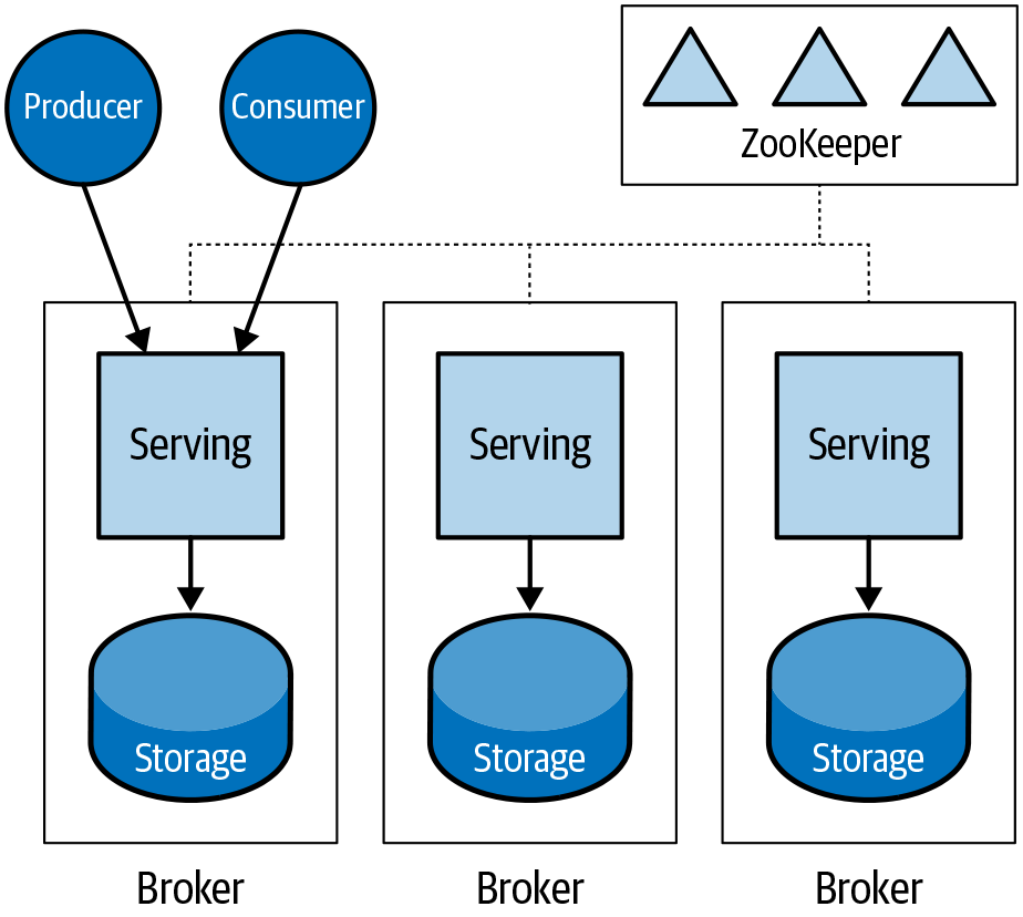
图 1. Kafka 架构图
Kafka Broker 承包了 Kafka 的所有消息功能,包括终止生产者和消费者连接、接受来自生产者的新消息并将消息发送给消费者。为了保证消息持久化,Broker 还为消息提供持久化存储功能。每个 Kafka Broker 负责一组主题。
Kafka Broker 是有状态的。每个 Broker 都存储了相关主题的完整状态,有了这些信息 Broker 才能正常运行。如果一个 Broker 发生故障,并不是任何 Broker 都可以接管它,而是必须拥有相关主题副本的 Broker 才能接管。如果一个 Broker 负载太高,也不能简单地通过增加 Broker 来分担负载,还需要移动主题(状态)才能平衡集群中的负载。虽然 Kafka 提供了用来帮助重平衡的工具,但是要用它来运维 Kafka 集群的话,你必须了解 Kafka Broker 与其磁盘上存储的消息状态的关系才行。
消息计算(Serving)是指消息在生产者和消费者之间的流动,在 Kafka Broker 中消息计算与消息存储是相互耦合的。如果你的使用场景中所有消息都能被快速地消费掉,那么对消息存储的要就可能较低,而对消息计算的要求则较高。相反,如果你的使用场景中消息消费得很慢,则需要存储大量消息。在这种情况下,对消息计算的要求可能较低,而对消息存储的要求则较高。
由于消息的计算和存储都封装在单个 Kafka Broker 中,所以无法独立地扩展这两个维度。即便你的集群只对消息计算有较高要求,你还是得通过添加 Broker 实现扩展,也就是说不得不同时扩展消息计算和消息存储。而如果你对消息存储有较高要求,而对消息计算的要求较低,最简单的方案也是添加 Kafka Broker,也就是说还是必须同时扩展消息计算和消息存储。
在扩展存储的场景中,你可以在现有的 Broker 上添加更多磁盘或者增加磁盘容量,但需要小心不要创建出一些具有不同存储配置和容量的独特 Kafka Broker。这种“雪花”(Snowflake)服务器环境比具有统一配置的服务器环境要复杂得多,更难以管理。
Pulsar
Pulsar 架构中主要有三个组件:ZooKeeper、Pulsar Broker 和 Apache BookKeeper Bookie,如图 2 所示。与 Kafka 一样,ZooKeeper 提供服务发现、领导者选举和元数据存储。与 Kafka 不同的是,Pulsar 通过 Broker 和 BookKeeper Bookie 组件分离了消息处理计算与消息存储功能。
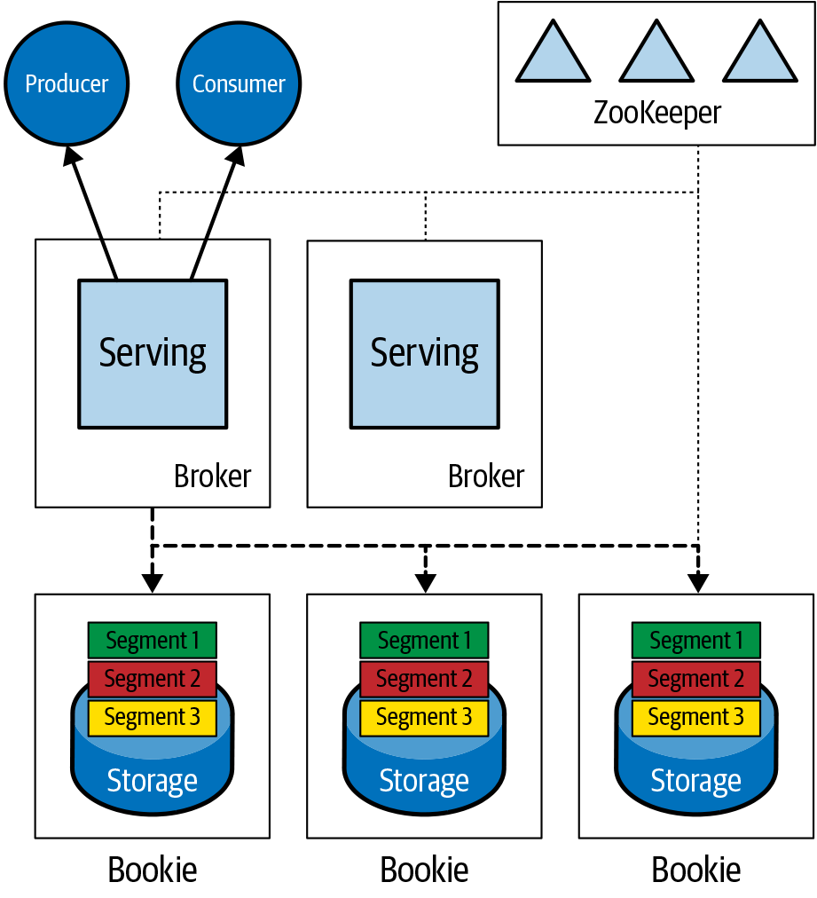
图 2. Pulsar 架构图
Pulsar Broker 负责消息计算,而 BookKeeper Bookie 负责消息存储。这是一种分层架构,Pulsar Broker 处理生产者和消费者之间的消息流动,而将消息存储交给 BookKeeper 层处理。
得益于这种分层架构,Pulsar Broker 是无状态的,这一点与 Kafka 不同。这意味着任何 Broker 均可接管失效的 Broker。也意味着新的 Broker 上线后可以立即开始处理生产者和消费者的消息流动。为了确保 Broker 之间的负载均衡,Pulsar Broker 内置了一套负载均衡器,不断监视每个 Broker 的 CPU、内存以及网络使用情况,并据此在 Broker 之间转移主题归属以保持负载均衡。这个过程会让 Latency 小幅增加,但最终能让集群的负载达到均衡。
BookKeeper 作为数据存储层当然是有状态的。提供可靠消息投递保证的消息系统必须为消费者保留消息,所以消息必须持久化存储到某个地方。BookKeeper 旨在构建跨服务器的分布式日志,它是一个独立的 Apache 项目,用于多种应用中,而非仅仅是 Puslar 中。
BookKeeper 将日志切分成一个一个被称为 Ledger 的分片(Segment),这样就很容易在 BookKeeper Bookie 节点之间保持均衡。如果 Bookie 节点故障,一些主题会变成小于复制因子(Under Replicated)。发生这种情况后 BookKeeper 会自动从存储与其他 Bookie 中的副本复制 Ledger,从而让其恢复到复制因子,而无需等待故障 Bookie 恢复或等待其他 Bookie 上线。如果添加一个新 Bookie,它能立即开始存储已有主题的新 Ledger。由于主题或分区并不从属于某个 Bookie,所以故障恢复过程无需将主题或分区移动到新服务器。
复制模型
为了保证消息持久性,Kafka 和 Pulsar 都对每个消息存储多个拷贝或副本。但是他们各自使用了不同的复制模型。
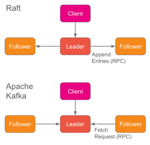
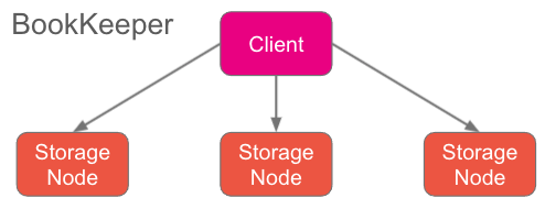
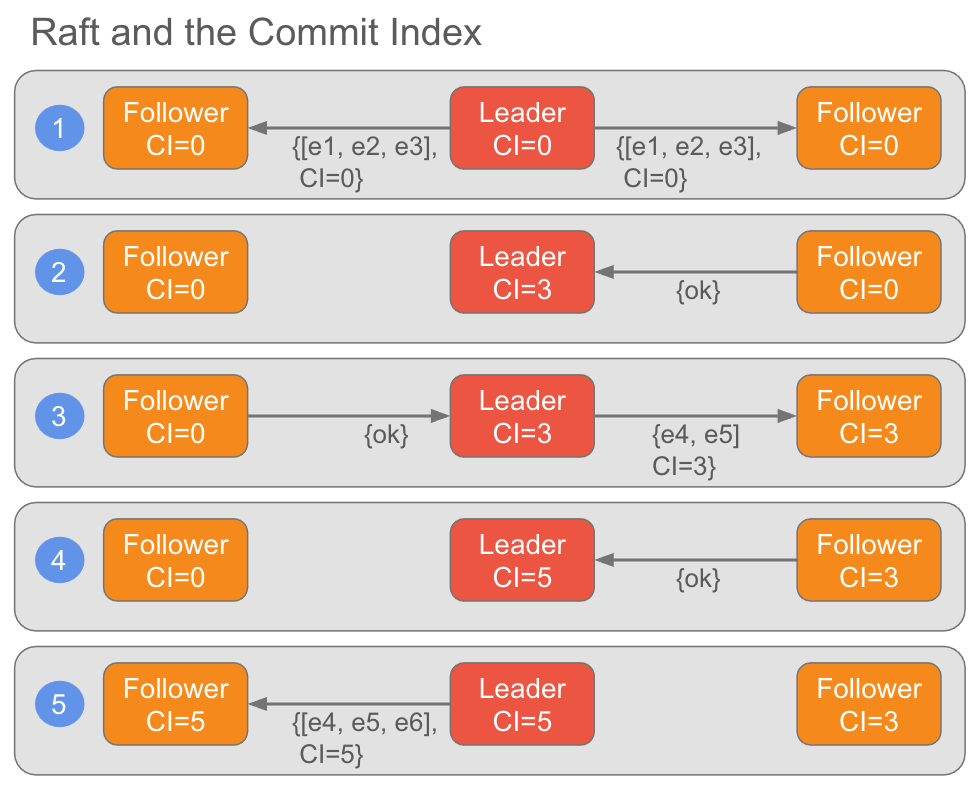
Kafka 使用的是 Leader-Follower 复制模型。对每个主题(确切说是主题分区,稍后我们会详细解释)都会选出一个 Broker 作为 Leader。所有消息最初都写入到 Leader,然后 Follower 从 Leader 读取并复制消息,如图 3 所示。这种关系是静态的,除非 Broker 发生故障。同一主题的消息总是被写入同一组 Leader 和 Follower Broker。引入新的 Broker 并不会改变现有主题的关系。
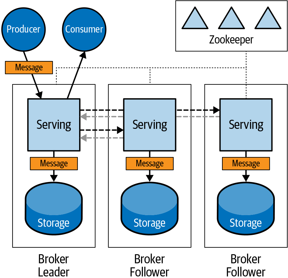
图 3. Kafka leader–follower 复制模型
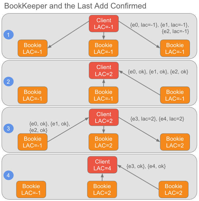
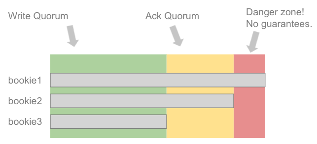
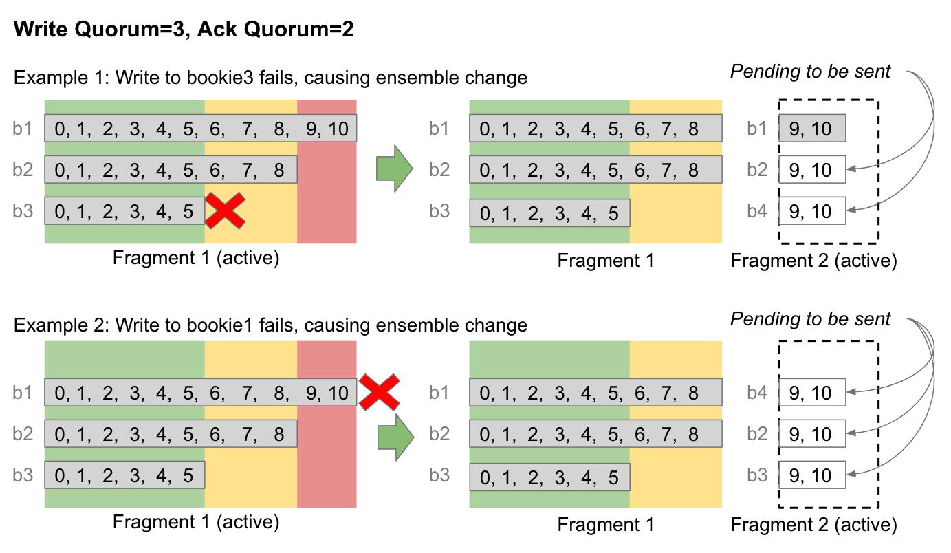
Pulsar 使用的则是法定人数投票复制模型(quorum-vote)。Pulsar 并行写入消息的多个副本(Write Quorum)。一旦一定数量的副本被确认写入成功,则该消息被确认(Ack Quorum)。与 Leader-Follower 模型不同,Pulsar 将副本分散(或称为条带化写入)到一组存储节点(Ensemble)中,这能改善读写性能。这也意味着新的节点添加成功后,即可立即成为可写入集合的一部分,用于存储消息。
如图 4 所示,消息被发往 Broker,然后被切分成分片(Segment)并写入多个 Bookie 节点。这些 Bookie 节点存储分片并发送确认给 Broker。一旦 Broker 从足够多的 Bookie 节点收到足够多的分片确认,则向生产者发送消息确认。
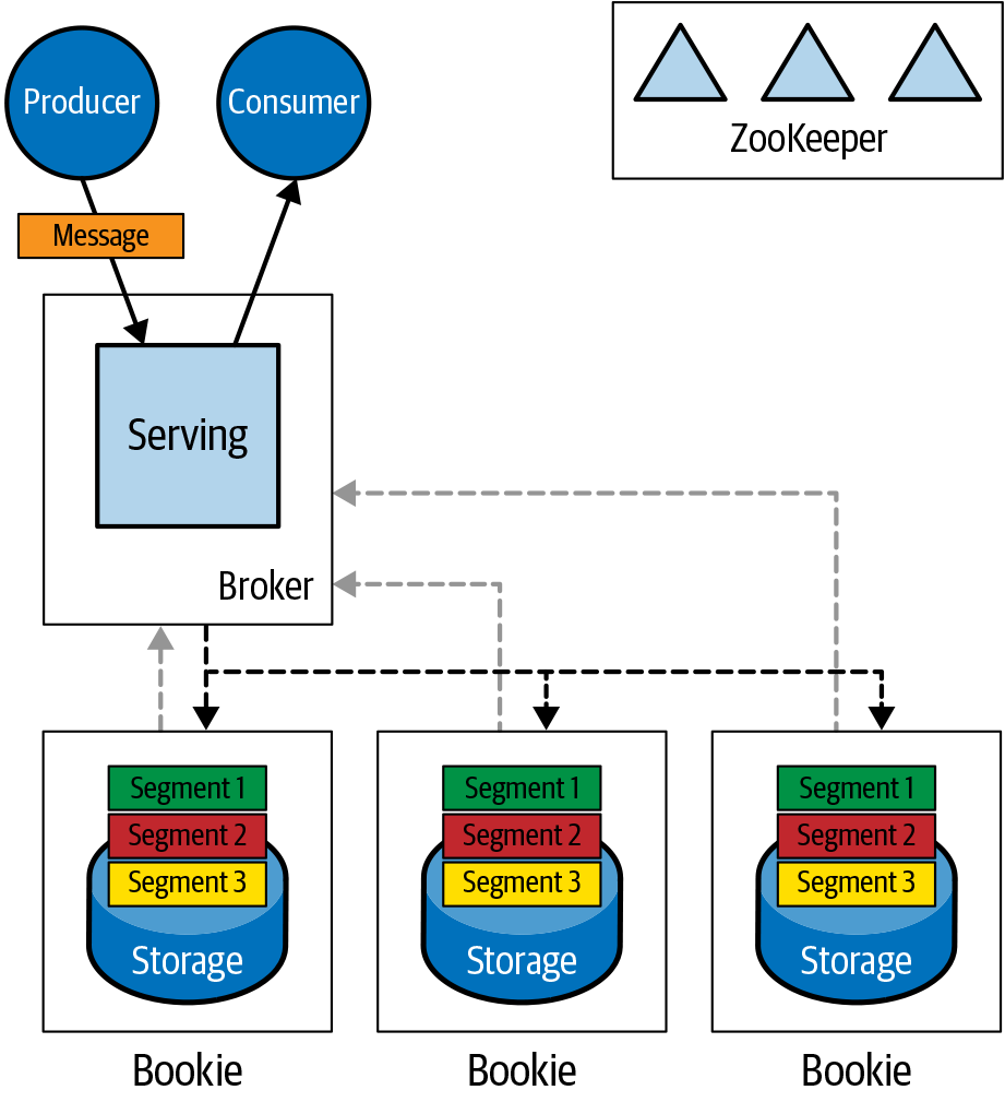
图 4. Pulsar quorum–vote 复制模型
由于 Broker 层是无状态的、存储层是分布式的、并且使用了法定人数投票复制模型(quorum-vote),所以与 Kafka 相比 Puslar 能更容易地处理服务器故障。只需替换掉故障服务器,Pulsar 即可自动恢复。增加新容量也更容易,只需简单的水平扩展即可。
而且由于计算层和存储层是分离的,所以你可以独立地扩展它们。如果对计算要求较高而对存储要求较低,那么在集群中加入更多的 Puslar Broker 即可扩展计算层。如果对存储要求很高而对计算要求很低,那么加入更多 BookKeeper Bookie 即可扩展存储层。这种独立的可扩展性意味着你可以更好地优化集群资源,避免在仅需要扩展计算能力时不得不浪费额外的存储,反之亦然。
Pub–Sub 消息系统概览
Kafka 和 Pulsar 支持的基础消息模式都是 pub-sub,又称发布订阅。在 pub-sub系统中,消息的发送方和接收方是解耦的,因此彼此透明。发送方(生产者)将消息发送到一个主题,而无需知道谁将接收到这些消息;接收方(消费者)订阅要接收消息的主题。发送方和接收方并不互相连接,且随时间推移可能变化。
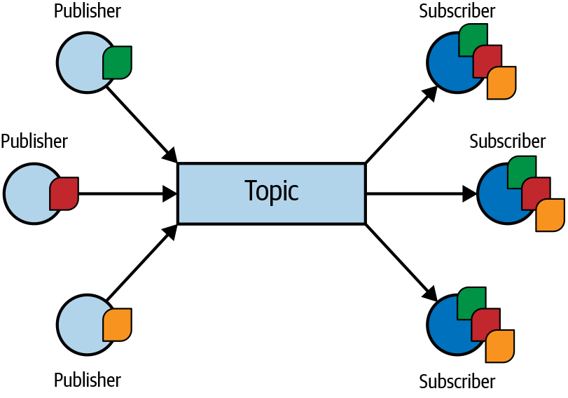
图 5. Pub–sub 消息模式:每个订阅者都能收到生产者发送的一条消息拷贝
Pub-sub 消息模式的一个关键特性是单个主题上可能有多个生产者与订阅者。如图 5 所示,多个发布应用可以发送消息到一个主题,多个订阅应用可以接收这些消息。重要的是,每个订阅应用都会收到自己的消息拷贝。所以如果发布了一条消息并且有 10 个订阅者,那么就会发送 10 条消息拷贝,每个订阅者收到一条消息拷贝。
Pub-sub 消息模式并不是什么新鲜事物,且被多种消息系统支持:RabbitMQ、ActiveMQ、IBM MQ,数不胜数。Kafka 与这些传统消息系统的区别在于,它有能力扩展到支持海量消息,同时保持一致的消息延迟。
与 Kafka 类似,Pulsar 也支持 pub-sub 消息模式,且也能支持海量消息且具有一致延迟。Kafka 使用消费者组来实现多个消费者接收同一消息的不同拷贝。Kafka 会与主题关联的每个消费者组发送一条消息。Pulsar 使用订阅(Subscription)来实现相同的行为, 向与主题关联的每个订阅发送一条消息。
日志抽象
Kafka 与传统消息系统的另一个主要区别是将日志作为处理消息的基本抽象。生产者写入主题,即写入日志;而消费者独立地读取日志。然而与传统消息系统不同,消息被读取后并不会从日志中删除。消息被持久化到日志中直至配置的时间到期。Kafka 消费者确认消息后并不会删除消息,而是提交一个偏移量值来表示它已读取了多少日志。此操作不会从日志中删除消息或以任何方式修改日志。总之,日志是不可变的。
为了防止日志变得无限长,日志中的消息在一段时间(保留周期)后会过期。过期的消息会从日志中删除。Kafka 默认的保留周期是七天。图 6 展示了发布的消息是如何附加到日志中,消费者如何以不同的偏移量读取它。日志中的消息到期后会过期并被删除。
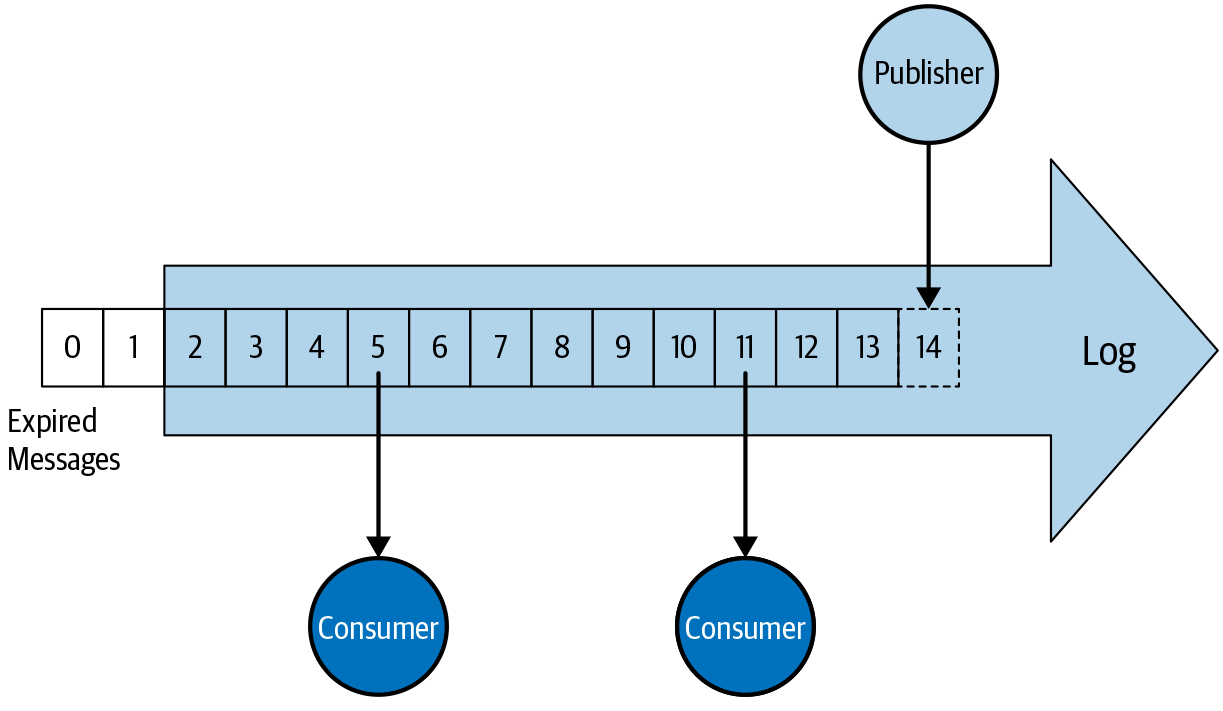
图 6. 日志抽象
消息重放
利用日志抽象可以允许多个消费者独立地读取同一个主题,同时还能支持消息重放。由于消费者只是从日志中读取消息并提交日志偏移量,因此只要将偏移量移动到较早位置就能很容易地让消费者重放已消费过的消息。支持消息重放有很多优势。例如,有 bug 的应用程序修复后可以重放之前消费过的消息以纠正其状态。在测试应用程序或开发新应用程序时,消息重放也很有用。
与 Kafka 类似,Pulsar 也使用日志来抽象其主题,只不过具体实现有所不同。这意味着 Puslar 也能支持消息重放。在 Puslar 中,每个订阅都有一个游标来跟踪其在主题日志中的消费位置。创建订阅的时候可以指定游标从主题的最早或最新消息开始读取。你可以将订阅游标倒回到特定消息或特定时间(例如倒回 24 小时)。
传统消息模型
到目前为止,我们看到 Kafka 与 Pulsar 有许多相似之处。他们都是能处理海量消息的 pub-sub 消息系统,都使用日志来抽象主题,并支持消息回放。不同之处在于对传统消息模型的支持。
在传统消息模型中,消息系统负责确保将消息投递给消费者。消息系统会跟踪消费者是否已经确认消息,并周期性地将未被确认的消息重新投递给消费者,直至被确认为止。一旦消息被确认,即可被删除(或标记为将来删除)。而未被确认的消息永远不会被删除,它将永远存在。而已确认的消息永远不会再发送给消费者。
Pulsar 利用订阅充分支持上述模型。 由于这种能力,Puslar 能够支持额外的消息模式,专注于消息如何被消费。
队列与竞争消费者
我们首先要分析的消息模式是传统队列模型。这种模型中队列消息代表一系列将要完成的工作(工作队列)。你可以使用单个消费者从队列中读取消息并执行工作,但更常见的做法是在多个消费者中分配工作。这种模式被称为竞争消费者模式,如图 7 所示。
在竞争消费者模式中,队列用于存储需要很长时间来处理的消息,例如转换视频。一条消息被发布到队列中后,被消费者读取并处理。当消息被处理完成后,消费者发回确认,然后消息从队列中删除。如果是单个消费者,则队列中的所有消息会被阻塞,直到消息被处理并确认。
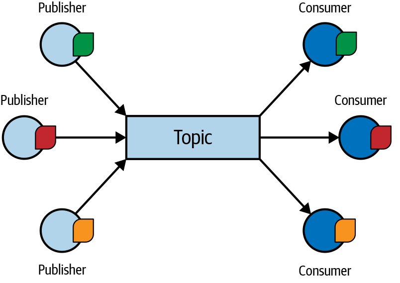
图 7. 竞争消费者:每条消息被一个消费者处理一次
为了改善整个流程并保持队列不被填满,你可以往队列中添加多个消费者。然后多个消费者会“竞争”从队列中获取消息并处理它们。如果上述视频转换的例子中我们有两个消费者,则相同时间内能处理的视频量会增加到两倍。如果这还不够快,我们可以添加更多消费者来提高吞吐量。
为了更有效,工作队列需要始终将消息分发给那些有能力处理队列消息的消费者。如果消费者有能力处理消息,则队列就将消息发给它。
Kafka
Kafka 使用消费者组和多分区来实现竞争消费者模式。Kafka 主题由一个或多个分区组成,消息被发布后通过 round-robin 或者消息 key 分布到主题分区中,随后被消费者组从主题分区中读取。
需要注意的是,Kafka 的一个分区一次只能被一个消费者消费。要实现竞争消费者模式,则每个消费者要有对应的分区。如果消费者数目多于分区数目,则多出来的消费者就会被闲置。举个例子,假设你的主题有两个分区,则消费者组中最多有两个活跃消费者。如果增加第三个消费者,则该消费者没有分区可以读取,所以不会竞争读取队列中的工作(消息)。
这意味着在创建主题时就需要明确有多少竞争消费者。当然你可以增加主题分区数,但这是相当重的变动,尤其当根据 key 分配分区时。除了 Kafka 消费者与主题的对应关系外,往消费者组中添加消费者会重平衡该主题的所有消费者,这种重平衡会暂停对所有消费者的消息投递。
所以说 Kafka 虽然确实支持竞争消费者消息模式,但是需要你仔细管理主题的分区数,确保添加新消费者时能真的处理消息。另外,与传统消息系统不同,Kafka 不会周期性地重新投递消息以便可以再次处理这些消息。如果想要有消息重试机制,你需要自己实现。
Kafka 确实比传统消息系统有个优势。竞争消费者模式的一个弊端是消息可能被乱序处理。因为竞争消费消息的多个消费者可能处理速率不同,很有可能消息会乱序处理。如果消息代表独立的工作,那么这不是什么问题。但如果消息代表像金融交易这样的事件,那有序性就很重要了。
由于 Kafka 分区一次只能被一个消费者消费,所以 Kafka 可以在竞争消费者模式下保证相同 key 的消息被顺序投递。如果消息是按照 key 路由到分区,则每个分区中的消息是按照发布的顺序存储的。消费者可以消费该分区并按顺序获取消息。这使得你可以扩展消费者以并行处理同时保持消息顺序,当然这一切都需要仔细的规划才行。
Pulsar
Pulsar 中的竞争消费者模式很容易实现,只需在主题上创建共享订阅即可。之后消费者使用此共享订阅连接到主题,消息以 round-robin 方式被连接到该订阅上的消费者消费。消费者的上线下线并不会像 Kafka 那样触发重平衡。当新的消费者上线后即开始参与 round-robin 消息接收。这是因为与 Kafka 不同,Pulsar 并不使用分区来在消费者之间分发消息,而完全通过订阅来控制。Pulsar 当然也支持分区,这一点我们稍后将讨论,但消息的消费主要是由订阅控制,而不受分区控制。
Pulsar 订阅会周期性地将未确认消息重新投递给消费者。不仅如此,Pulsar 还支持高级确认语义,例如单条消息确认(选择性确认)和否定确认(negative acknowledgment),这一点对工作队列场景很有用。单条消息确认允许消息不按顺序确认,所以慢速消费者不会阻塞对其他消费者投递消息,而累积确认是可能发生这种阻塞的。否定确认允许消费者将消息放回主题中,之后可以被其他消费者处理。
Pulsar 支持按 key 将消息路由到分区,所以也可以使用与 Kafka 一样的方案来实现竞争消费者。共享订阅这种实现方式更加简单,但是如果你想在横向扩展消费者并行处理能力的同时也保证按 key 有序,Pulsar 也是可以实现的。
Pulsar 订阅模型
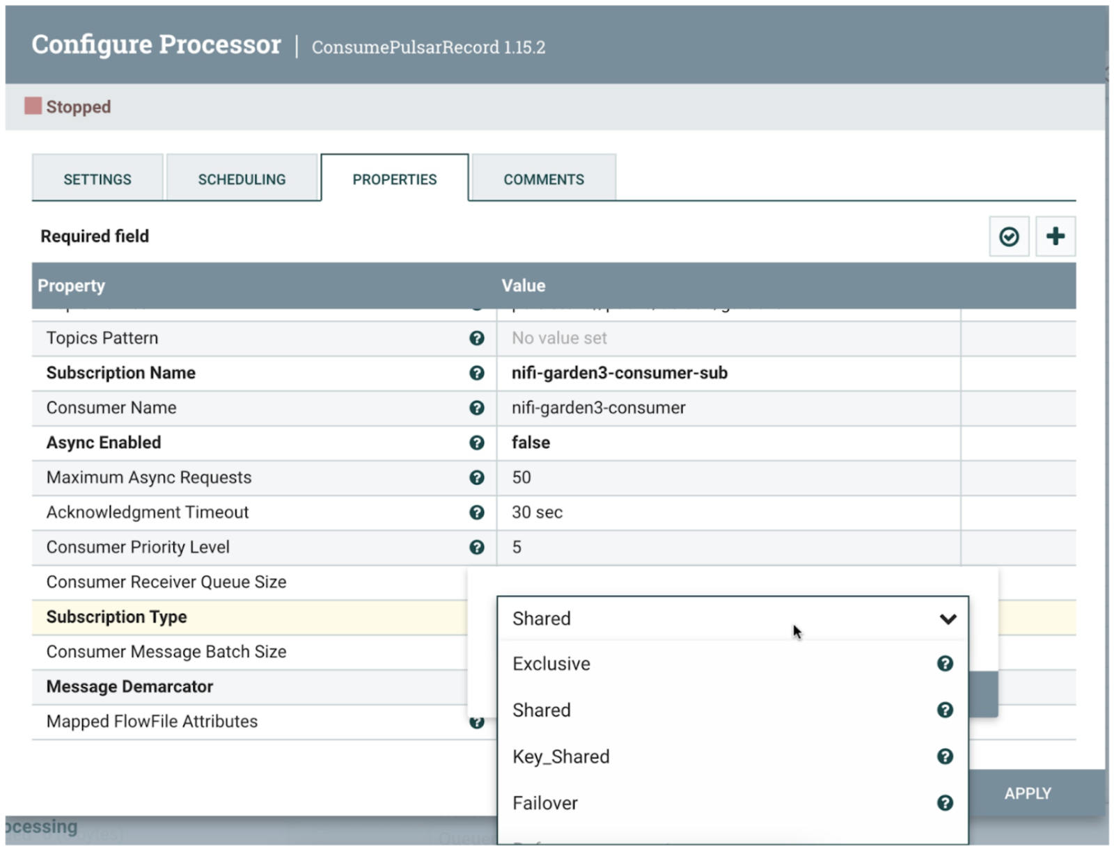
共享订阅是 Pulsar 中实现工作队列的一种简单方式。Puslar 还支持其他订阅模型来支持多种消息消费模式:独占、 灾备、共享、键共享,如图 8 所示。
独占订阅模型中,不允许超过一个消费者消费主题消息。如果其他消费者尝试消费消息,则会被拒绝。如果你需要保证消息被单个消费者按顺序消费,那就使用独占订阅模型。
灾备订阅模型中,允许多个消费者连接到一个主题,但是在任何时间都只有一个消费者可以消费主题。这就建立了一种主备关系,一个消费者处于活跃状态,其他的处于备用状态,当活跃消费者故障时进行接管。当活跃消费者断开连接或失败,所有未确认消息会被重新投递到某个备用消费者。
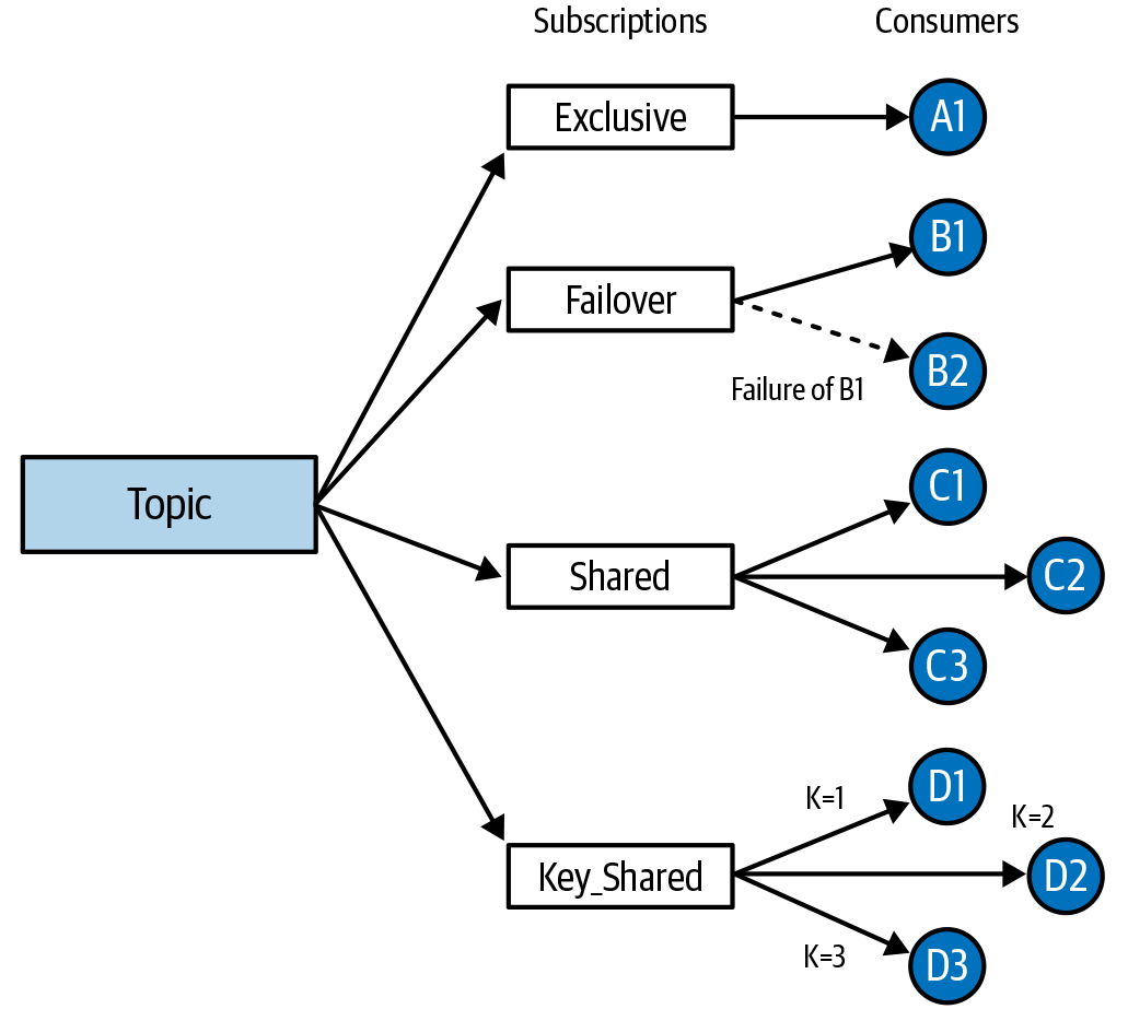
图 8. Pulsar 订阅模型:独占、灾备、共享、键共享
前文已提到,基于共享订阅模型实现的竞争消费者模式的一个弱点是消息可能被乱序处理。在 Kafka 和 Pulsar 中,都可以通过将消息按 key 路由到分区来解决。Puslar 最近推出了一种新的名为 key_shared 的订阅模型,可以更简单地解决这个问题。这种订阅模式的优点是可以按 key 有序投递消息而无需关心分区。消息可以发布到单个主题并分发给多个消费者,这跟共享订阅模型一样。不一样的是,单个消费者只会接受对应某个 key 的消息。这种订阅模型可以通过 key 按顺序投递消息而无需对主题进行分区。
Pulsar:整合 Pub–Sub 与队列
如我们所见,Kafka 和 Pulsar 都支持 pub-sub 消息投递。它们都使用日志来抽象主题,所以可以支持重放已被消费者处理过的消息。但是 Kafka 只能有限地支持按不同方式来消费消息,不会自动重新投递消息,也不能保证未确认的消息不会丢失。实际上,保留周期之外的所有消息无论是否被消费过都会被删除。Kafka 可以实现工作队列,但有很多事项需要注意和考虑。
由于这些限制,如果企业需要高性能 pub-sub 消息系统、同时需要可靠性投递保证以及传统消息模式,他们通常会在 Kafka 之外使用传统的消息系统,例如 RabbitMQ。将 Kafka 用于高性能 pub-sub 场景,而将 RabbitMQ 用于要求可靠性投递保证的场景,例如工作队列。
Pulsar 在单个消息系统中同时支持高性能 pub-sub 以及保证可靠性投递的传统消息模式。在 Pulsar 中实现工作队列非常简单——实际上这也是 Puslar 最开始设计时就想解决的场景。如果你正同时使用多个消息系统——使用 Kafka 处理高流量 pub-sub场景、使用 RabbitMQ 处理工作队列场景——那么可以考虑使用 Puslar 把它们整合成单个消息系统。即便最初只有一种消息场景需求,也可以直接使用 Pulsar 以应对未来可能出现的新的消息场景。
运维单个消息系统显然要比运维两个要更加简单、所需的 IT 和人力资源也更少。
日志抽象
现在我们介绍了 Kafka 与 Puslar 的高层次架构,也了解了这两个系统能实现的各种消息模式,接下来让我们更详细地了解这两个系统的底层模块。首先我们来看看日志抽象。
Kafka 团队的设计思路值得称赞,日志的确是实时数据交换系统的一个很好的抽象。因为日志只能追加,所以数据可以快速写入;因为日志中的数据是连续的,所以可以按照写入顺序快速读取。数据的顺序读写是很快的,而随机读写则不然。在提供数据保证的系统中,持久化存储交互都是瓶颈,而日志抽象则让这一点变得尽可能高效。Kafka 和 Pulsar 都使用日志作为其底层模块。
为了简单起见,下文假设 Kafka 主题是单分区的,因此下文中主题和分区是同义词。
Kafka 日志
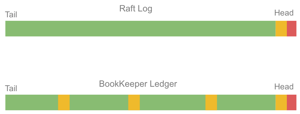
在 Kafka 中,每个主题都是一个日志。日志作为单个存储单元存储在 Kafka Broker 上。虽然日志由一系列文件组成,但日志并不能拆分到多个 Broker 上,也不能拆分到同一个 Broker 的多个磁盘上。这种将整个日志作为最小存储单元的方式通常运行良好,但是当规模增大或在维护期间会很麻烦。
比方说日志的最大大小会受其所在磁盘容量的限制。因此,存储日志的 Broker 磁盘大小限制了主题的大小。在 Broker 上添加磁盘并不能解决问题,因为日志是最小存储单元,并不能跨磁盘拆分。唯一的选择是增加磁盘大小。这在云环境中是可行的,但如果你在物理硬件上运行 Kafka,那么增加现有磁盘的容量不是一件容易的事。
还有另一件麻烦的事,由于日志与其底层文件是一对一绑定的,所以在实时系统上执行维护操作是很麻烦的。如果 Broker 服务器出现故障,或者需要增加新的 Broker 来分担高负载,都需要在服务器之间拷贝大量日志文件。在保持数据实时性的同时执行大量文件拷贝会给 Kafka 集群带来很大压力。
Pulsar 分布式日志
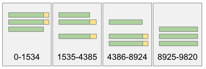
与 Kafka 一样,Apache Pulsar 也使用日志抽象作为其实时消息系统的基础,每个主题在 Pulsar 中也是一个日志。然而 Pulsar 采用不一样的方式将日志写入存储。Pulsar 不是将日志作为最小存储单元存储到单个服务器,而是将日志分解为分片(或称为 Ledger),然后将 Ledger 分布到多个服务器。通过这种方式,Pulsar 创建的分布式日志驻留在多个服务器上。
分布式日志有许多优点。日志的最大大小不再受限于单个服务器的磁盘容量。由于分片是跨服务器分布的,所以日志可以增长到所有服务器的总存储容量一样大。增加分布式日志的容量就像往集群添加服务器一样简单。一旦新服务器上线,分布式日志即可开始使用新上线的容量来写入新的日志分片。也无需调整磁盘大小或重平衡分区来分配负载了。一旦服务器出现故障,故障恢复也很简单。故障丢失的分片可以从多个不同的服务器恢复出来,从而缩短恢复时间。
显而易见,让分布式日志可靠地工作起来是很困难的。这也是为什么 Puslar 要使用另一个 Apache 项目(BookKeeper)来实现分布式日志的原因。要运行 Pulsar 的话必须同时运行 Apache BookKeeper 集群。尽管这会引入运维复杂度,但是 BookKeeper 这个分布式日志的底层组件已经过验证且被广泛应用。BookKeeper 专为健壮的、低延迟的读写而设计。举个例子,BookKeeper 从架构上将写入和读取分离到单独的磁盘,这样一来慢速消费者就不会影响生产者发布新消息的性能。
BookKeeper 还为 Puslar 提供高持久性保证。当消息存储到 BookKeeper 时,会先刷到磁盘再给生产者发回确认;即便 BookKeeper 服务器故障,所有已确认的消息仍然能保证永久存储在磁盘上。BookKeeper 能够在保持低延迟的同时提供这种高持久性保证。
反观 Kafka,默认情况下定期将消息刷到磁盘。这意味着 Kafka Broker 发生故障后几乎总会导致消息丢失,因为这些消息尚未被刷到磁盘。当然,通过配置在线副本数,这些丢失的消息可以恢复;但是 BookKeeper 服务器发生类似故障的情况下,不会有数据丢失,所以也就不需要数据恢复。Kafka 也可以配置为将每条消息即时刷到磁盘,但这会带来性能损失。
多级存储
Pulsar 存储计算分离的另一个优点是允许在架构中引入第三层,即长期存储,又称冷存储。Pulsar 和 BookKeeper 针对快速访问主题中的消息进行了优化;然而,如果你的消息量非常大但不需要快速访问,或者只需要快速访问最新的消息即可,那么 Pulsar 允许你将这些消息推送到云对象存储,例如 AWS S3 或者 Google Cloud Storage。Pulsar 是这样实现该功能的:将主题中的老分片卸载(offload)到云提供商,然后从 bookie 本地存储中删除这些消息。
云对象存储比起构建高性能消息系统常用的高速 SSD 磁盘要便宜得多,因此运营成本也更低。由于云存储提供了几乎无限的存储容量,所以你不必担心超出你集群的存储容量。非常大的主题可能主要驻留在云存储中,而其他较小的主题则驻留在 bookie 节点的高速磁盘。
这种三层架构可以很好地适应需要永久存储消息的场景,比方说事件溯源。事件溯源是将所有状态变化都记录为事件,存储为 Pulsar 中的消息。应用的当前状态是由直到当前时间为止的整个事件历史记录确定。为了确保可以重建当前状态,你必须保存完整的事件历史。得益于持久性保证、使用分层存储实现近乎无限的存储容量,以及重放主题中所有消息的能力,Pulsar 非常适合事件溯源应用架构。
分区
如果你用过 Kafka,那么对分区一定很熟悉。本文中已经多次提及分区,因为这是绕不过去的。分区是 Kafka 中的一个基本概念,非常有用。Pulsar 也支持分区,但是是可选的。
Kafka 分区
Kafka 的所有主题都是分区的。一个主题可能只有一个分区,但必须至少有一个分区。分区在 Kafka 中是很重要的,因为分区是 Kafka 并行度的基本单元。将负载分散到多个分区即可分散到多个 Broker,单个主题的处理速度就能提高。Kafka 旨在处理高吞吐量,特别是要使用商用硬件来达到这个目的,分区在其中扮演着不可或缺的角色。
自 Kafka 诞生以来,商用硬件的容量不断提升。此外运行 Kafka 的 Java 虚拟机性能也不断提升。 这种硬件和软件的提升意味着现在在商用硬件上使用单分区也可以获得良好的性能。从性能角度来看,单分区主题也足以满足很多使用场景。
然而,正如前文所述,如果你想用多个消费者读取 Kafka 主题,就不能使用单分区。因为分区是 Kafka 生产和消费并行度的基本单元。因此即便单个分区足以满足主题的输入消息速度,你也希望使用多分区,以便将来可以选择增加多个消费者。当然,你也可以在创建主题之后再增加分区,但如果使用基于 key 的分区,这将会改变哪些 key 分配给哪些分区,从而影响分区中消息的处理顺序;而且分区会消耗资源(例如 Broker 上的文件句柄、客户端的内存占用),所以增加分区绝非一个轻量操作;另外虽然可以增加主题分区,但永远不能减少主题分区数。
正因为分区是 Kafka 的基础,所以要想用好 Kafka 就必须理解分区的工作原理。在创建主题时,你就需要考虑需要(或将来可能需要)多少分区数;在连接消费者时,你需要理解消费者如何与消费者组中的分区进行交互;如果你运维一个 Kafka 集群,一切都以分区级别运行,在维护和维修时,你需要以分区为中心。
Pulsar 分区
Pulsar 也支持分区,但是它们完全是可选的。事实上运行 Pulsar 时完全可以不使用分区。不分区的主题即可支持发布海量消息并支持多个消费者读取。如果你需要额外的性能,或需要基于 key 的有序消息消费,那么可以创建 Pulsar 分区主题。Pulsar 完全支持分区,其功能与 Kafka 大体相同。
Pulsar 分区被实现为一组主题的集合,用后缀来表示分区编号。例如创建一个包含三个分区的主题 mytopic,则会自动创建三个主题,分别名为 mytopic-parition-1、mytopic-partition-2 和 mytopic-partition-3。生产者可以连接到主主题 mytopic,根据生产者定义的路由规则将消息分发到分区主题。也可以直接发布到分区主题。同样地,消费者可以连接到主主题,也可以连接到一个分区主题。与 Kafka 一样,可以增加主题的分区数,但永远不能减少分区数。
由于分区在 Pulsar 中是可选的,所以 Pulsar 使用起来更加简单,尤其对于初学者来说。在 Pulsar 中你可以放心地忽略分区,除非你的使用场景需要用到分区提供的功能。这不仅简化了 Pulsar 集群的运维,也使得 Pulsar 客户端 API 更容易使用。分区是个有用的概念,不过如果你无需处理分区即可满足需求,那就有助于简化固有的复杂技术。
性能
Kafka 以其性能而闻名,以能够在实时环境中支持海量消息而著称。比较消息系统之间的性能有点棘手,每个系统都有性能最佳点和性能盲点,很难进行公平的比较。
OpenMessaging 项目 是一个旨在公平比较消息系统之间性能的项目,它是一个 Linux 软件基金会协作项目。OpenMessaging 项目由多个消息系统供应商支持,其目标是为消息和流系统提供供应商中立和语言独立的标准。该项目包含一个性能测试框架,支持多种消息系统,包括 Kafka 和 Pulsar。
其思想是利用标准的测试框架和方法,在评估中引入一定程度的公平性。OpenMessaging 项目的所有代码都是开源的,任何人都可以运行基准测试并输出自己的结果。
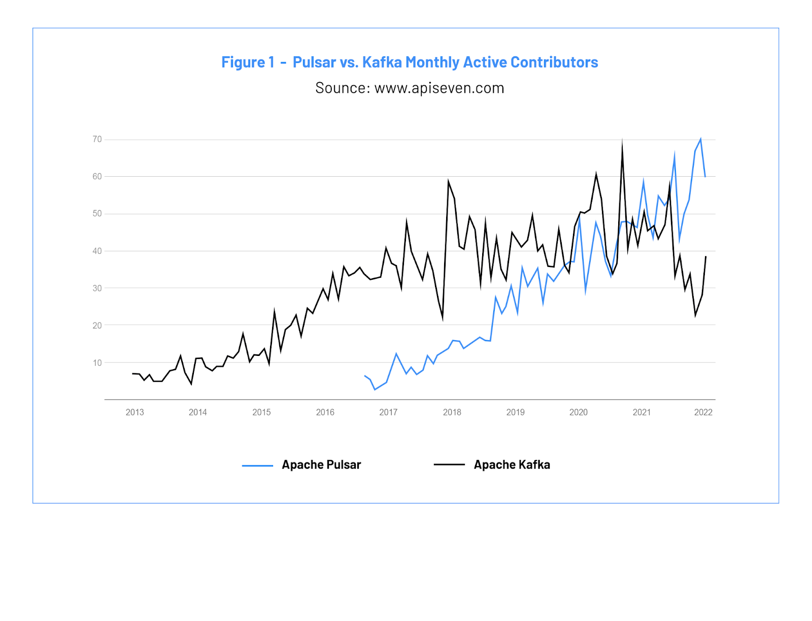
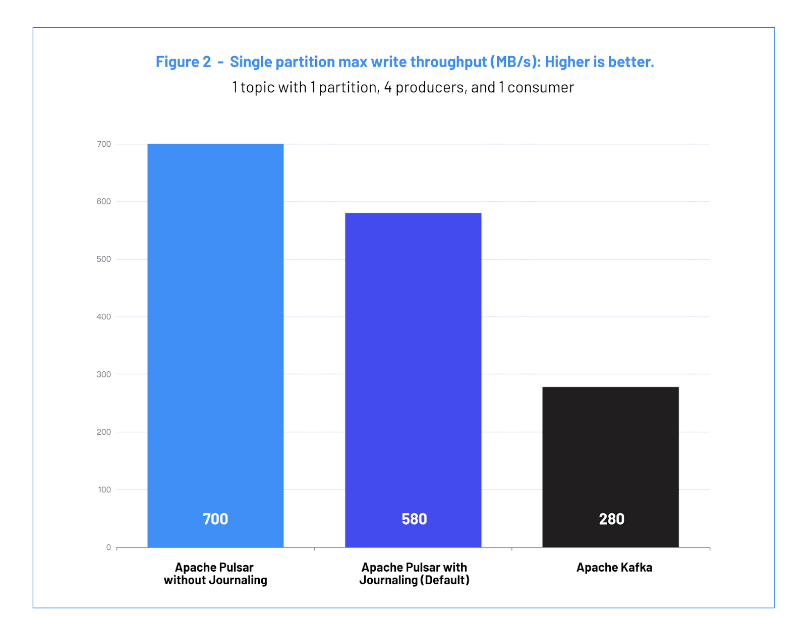
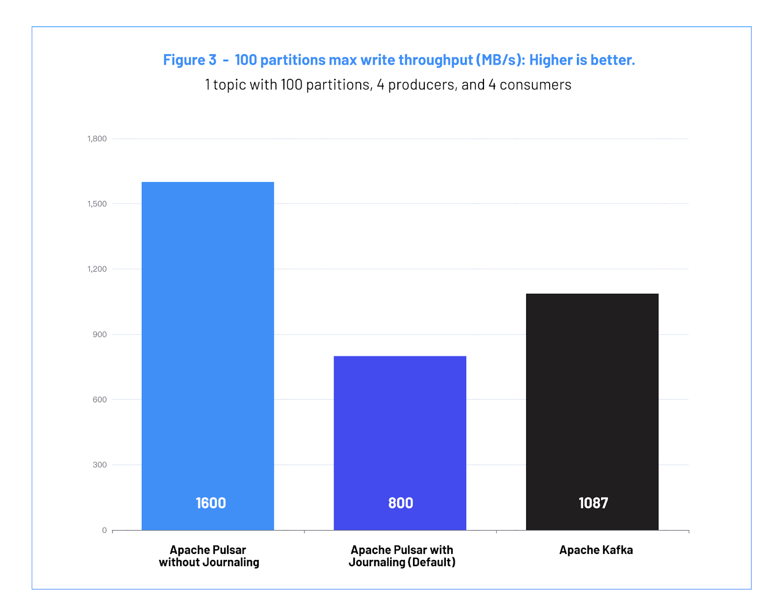
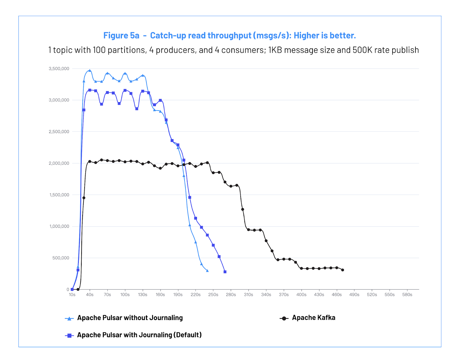
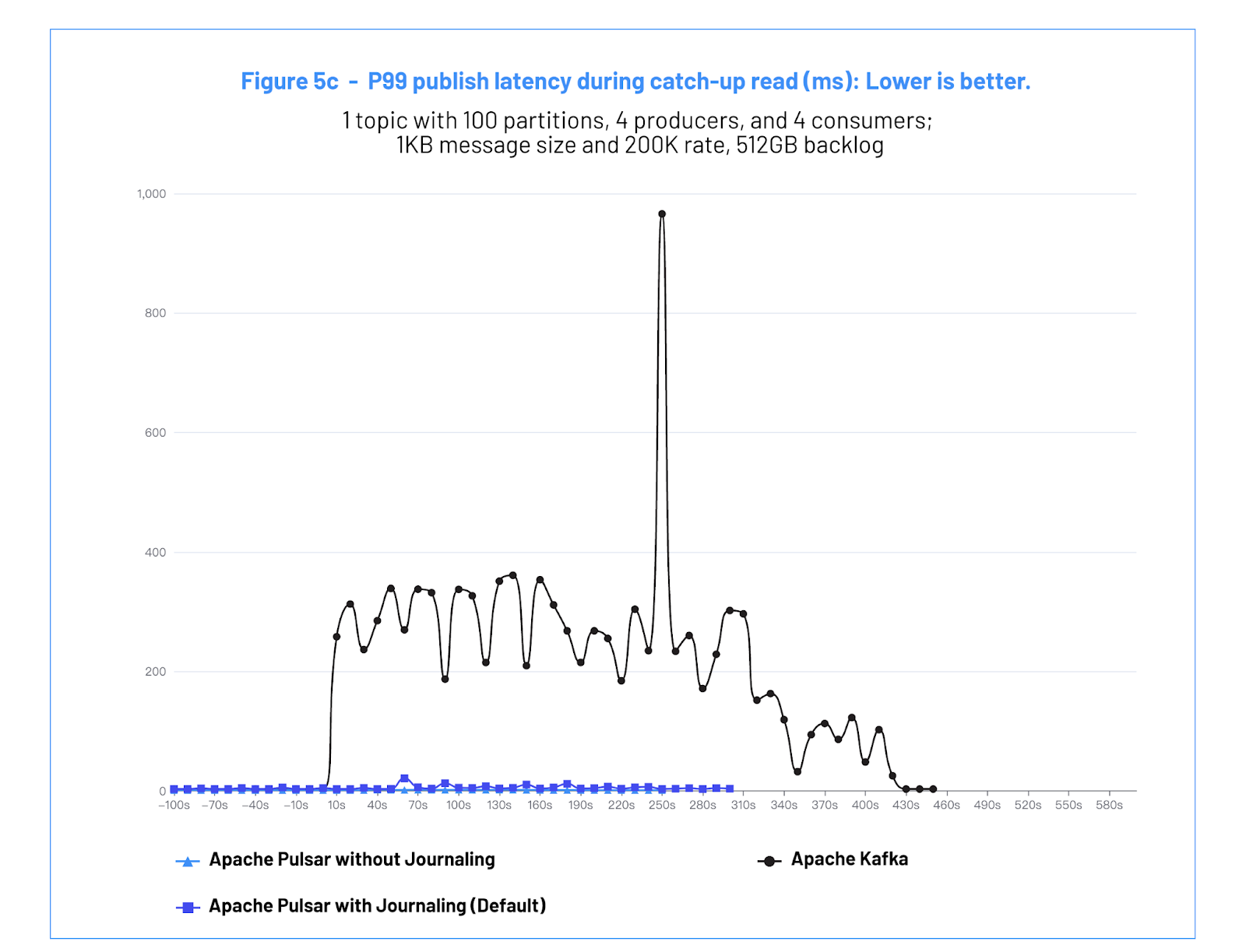
对 Kafka 和 Pulsar 进行详细的性能分析已经超出了本文的范围。不过一些基于 OpenMessaging 基准测试框架的测试结果表明 Pulsar 的性能要优于 Kafka。
GigaOm 发布的一份报告显示:
- Pulsar 的最大吞吐量高出 150%
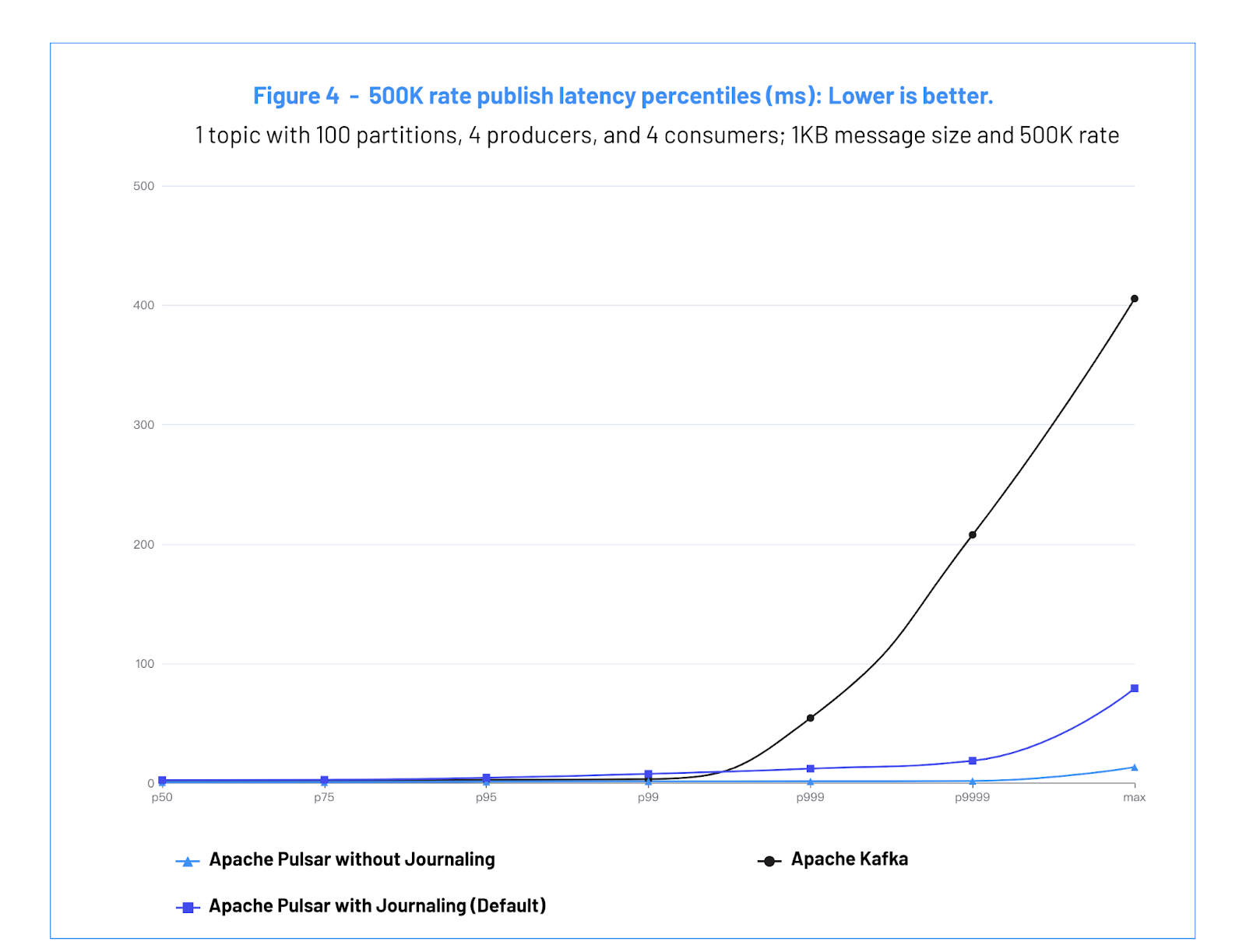
- Pulsar 的消息延迟降低了 40%,且更加稳定
- Pulsar 扩展性更好,在不同消息大小和分区数量下均能提供一致的结果
为了验证其中一些结果,我使用 OpenMessaging 项目的基准框架对 Kafka 和 Pulsar 的延迟进行了一个 详细对比。在这次对比中,我得出的结论是 Pulsar 能提供更加可预测的延迟。在许多情况下,Pulsar 的延迟比 Kafka 更低,尤其是在需要强持久性保证场景下,或需要大量分区的场景下。
多租户
租户是指可以独立使用系统的用户或用户组数量。在单租户系统中,所有的资源都是共享的,因此系统用户需要知道系统的其他用户在做什么。由于资源是共享的,必然引入争用和可能的冲突。如果多个用户组使用单租户系统,那么通常需要为系统提供多个拷贝,每个用户组使用一个拷贝,以提供隔离性和隐私。
在多租户系统中,不同的用户组或租户可以独立地使用系统。每个租户都是与其他租户隔离的。系统资源被各租户割据,所以每个用户都有自己的系统私有实例。我们只需提供一套系统,但每个租户都有自己的虚拟隔离环境。多租户系统可以支持多个用户组。
消息系统是一种核心基础设施,它最终会被多个不同的团队用于不同的项目。如果为每个团队或项目都创建一个新集群,那么运维复杂度会很高,而且也不能有效地利用资源。因此,多租户在消息系统中是一个令人向往的特性。
Pulsar
多租户是 Pulsar 的关键设计要求。因此 Pulsar 有多种多租户特性,让单个 Puslar 系统可以支持多个团队以及多个项目。
在 Pulsar 中,每个租户有自己的虚拟消息环境,与其他租户隔离开。一个租户创建的主题也与其他租户创建的主题隔离。通常,一个租户可以被一个团队或部门的所有成员使用。每个租户可以有多个命名空间。命名空间包含一组主题。不同命名空间可以包含同名的主题。命名空间可以便捷地将特定项目中的所有主题组织到一起。
命名空间也是一种在主题之间共享策略配置的机制。举个例子,所有需要 14 天保留周期的主题可以归到同一命名空间。在命名空间上配置该保留周期策略后,该命名空间内的所有主题都将继承这个策略。
当多个租户共享同一资源时,很重要的一点是要有某种机制确保所有租户都能公平地访问。需要确保一个租户不会消耗掉所有资源,导致其他租户饥饿。
Pulsar 有多种策略确保单个租户不至于消耗掉集群里的所有资源,例如限制消息出站速率、限制未确认消息存储以及限制消息保留期。可以在命名空间级别设置这些策略,这样各个主题组可以有不同的策略。
为了让多租户更好地工作,Pulsar 支持命名空间级别的授权。这意味着你可以限制对命名空间中主题的访问,可以控制谁有权限在命名空间中创建主题,以及谁有权限生产和消费这些主题。
Kafka
Kafka 是单租户系统,所有主题都属于一个全局命名空间。诸于保留周期等策略可以设置全局默认值,或者在单个主题上进行覆盖。但无法将相关主题组织到一起,也无法将策略应用到一组主题上。
关于授权,Kafka 支持访问控制列表(ACL),允许限制谁可以从主题上生产和消费。ACL 允许对集群中的授权进行细粒度的控制,可以对各种资源设置策略,比如集群、主题和消费者组;还可以指定各种特定的操作,比如创建、描述、更改和删除。除了基于用户(主体)的授权之外,还支持基于主机的授权。例如你可以允许 User:Bob 读写某个主题,但限制只能从 IP 地址 198.51.100.0 进行读写。而 Pulsar 没有这种细粒度的授权以及基于主机的限制,只支持少数几个操作(管理、生产、消费),并且不提供基于主机的授权。
尽管 Kafka 在授权控制上有更大的灵活性,但它本质上仍然是一个单租户系统。如果多个用户组使用同一个 Kafka 集群,他们需要保证主题名称不要冲突,并且 ACL 被正确应用。而多租户在 Pulsar 中是内置的,因此在不同团队和项目之间共享集群是非常简单的。
跨地域复制
Kafka 和 Pulsar 这类系统要实现高性能,重要一点是让其中的组件互相靠近以便有较低的互相通讯时延。这意味着 Kafka 和 Pulsar 要部署在单个数据中心,组件之间由高速网络互联。当集群内一个或多个组件(计算、存储、网络)发生故障时,集群内的消息复制机制保证免受消息丢失和服务宕机之苦。在云环境中,组件可以分布到一个数据中心(区域)内的多个可用区,以防止一个可用区发生故障。
但如果整个数据中心发生故障或被隔离,那么消息系统则会发生宕机(或发生灾难时丢失数据)。如果这对你来说不可接受,那么你可以使用跨地域复制。跨地域复制是指将消息复制到远端的另一个集群,发布到数据中心的每条消息都会被自动且可靠地复制到另一个数据中心。这可以防止整个数据中心发生故障。
跨地域复制对于全球应用程序来说也非常有用,消息从世界上某个位置生产出来,并被世界上其他地方的消费者消费。通过将消息复制到远程数据中心,可以分散负载,并提高客户端响应能力。
Pulsar
雅虎的团队在构建 Apache Pulsar 之初,一个关键需求就是要支持在跨地域的数据中心之间复制消息,需要确保即便整个数据中心发生故障消息仍然可用。因此对于 Pulsar 来说跨地域复制是一项核心功能,完全集成到管理界面中。可以在命名空间级别开启或关闭跨地域复制功能。管理员可以轻松配置哪些主题需要复制,哪些不需要复制。甚至生产者在发布消息时可以排除某些数据中心让它不接收消息复制。
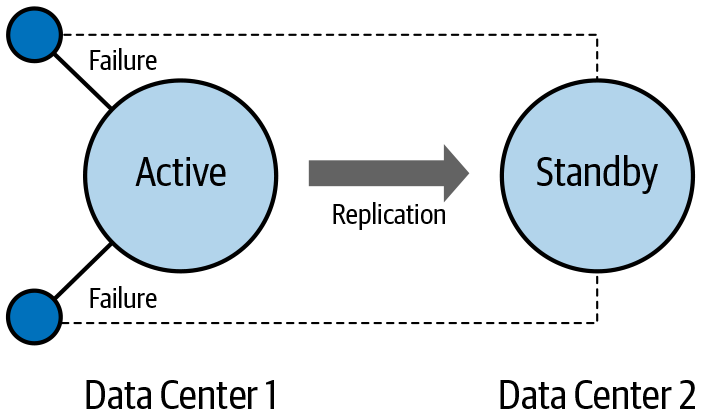
图 9. Active–standby 复制
Pulsar 的跨地域复制支持多种拓扑结构,例如主备(active-standby)、双活(active-active)、全网格(full mesh)以及边缘聚合(edge aggregation)。图 9 展示的是 active-standby 复制。所有消息都被发布到主数据中心(Data Center 1),然后被复制到备用数据中心(Data Center 2),如果主数据中心发生故障,客户端可以切换到备用数据中心。对于主备复制拓扑,Pulsar 新近引入了复制订阅(replicated subscription)功能,该功能在主备集群之间同步订阅状态,以便应用程序可以切换到备用数据中心并从中断的地方继续消费。
在主备(active–standby)复制中,客户端一次只连接到一个数据中心。而在双活(active-active)复制中,客户端连接到多个数据中心。图 10 所示的事一个全网格配置的双活复制拓扑。发布到一个数据中心的消息会被同步到其他多个数据中心。
图 11 所示的是边缘聚合拓扑(edge aggregation)。在此拓扑中,客户端连接到多个数据中心,这些数据中心将消息复制到中央数据中心进行处理。如果边缘数据中心处于客户端附近,那么即使中央数据中心离得很远,已发布的消息也能快速被确认。
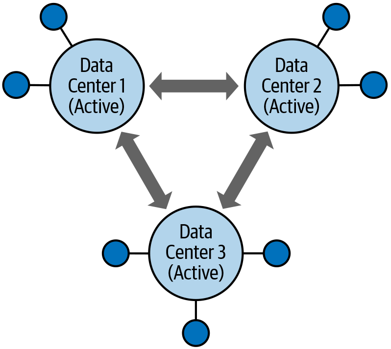
图 10. Active–active, full-mesh replication
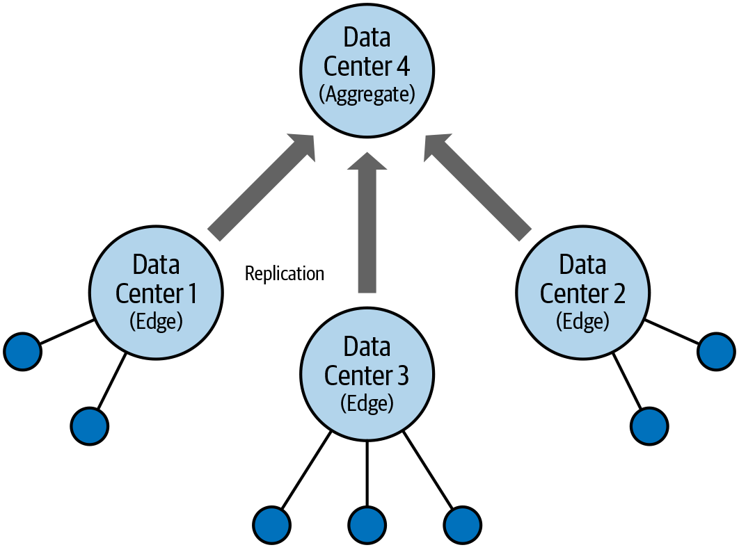
图 11. Edge aggregation
Pulsar 也可以进行同步跨地域复制。在典型的跨地域复制配置中,消息复制是异步完成的。生产者将消息发送到主数据中心后,消息即被持久化并确认回生产者;然后再被可靠地复制到远端数据中心。整个过程是异步的,因为消息在被复制到远端数据中心之前已向生产者确认。只要远端数据中心可用并且可以通过网络访问,这种异步复制就没有任何问题。然而,如果远端数据中心出现问题,或者网络连接变慢,那么已确认的消息就可能不能马上被复制到远端数据中心。如果主数据中心在消息被复制到远端数据中心之前发生故障,那么消息可能会丢失。
如果这种消息丢失对你来说不可接受,那么可以配置 Pulsar 进行同步复制。在同步复制时,消息直到被安全地存储到多个数据中心之后才会确认回生产者。由于消息要发到多数距离分散的数据中心,而数据中心之间有网络延迟,因此同步复制确认消息的时间会更长一些。不过这保证了即便整个数据中心故障也不会发生消息丢失。
Pulsar 有着丰富的跨地域复制功能,能支持几乎所有你能想到的配置。跨地域复制的配置和管理完全集成到 Pulsar 中,无需外部包也无需扩展。
Kafka
Kafka 中有多种方式可以实现跨地域复制,或者像 Kafka 文档那样称之为 mirroring。Kafka 提供了一个 MirrorMaker 工具,用来在消息生产后将其从一个集群复制到其他集群。这个工具很简单,只是将一个数据中心的 Kafka 消费者与另一个数据中心的 Kafka 生产者连接起来。它不能动态配置(改变配置后需要重启),且不支持在本地和远端集群机制同步配置信息或同步订阅信息。
另一个跨地域方案是由 Uber 开发并开源的 uReplicator。Uber 之所以开发 uReplicator 是为了解决 MirrorMaker 的许多缺点,提高其性能、可扩展性和可运维性。无疑 uReplicator 是更好的 Kafka 跨地域复制方案。然而它是一个独立的分布式系统,有控制器节点和工作节点,需要与 Kafka 集群并行运维。
Kafka 中还有用于跨地域复制的其他商业解决方案,例如 Confluent Replicator。它支持双活(active-active)复制,支持在集群间同步配置,并且比 MirrorMaker 更容易运维。它依赖于 Kafka Connect,需要与 Kafka 集群并行运维。
在 Kafka 中是可以实现跨地域复制的,但做起来并不简单。必须在多个方案中做出选择,需要并行运维各种工具,甚至并行运维整个分布式系统;所以说 Kafka 跨地域复制是很复杂的,尤其与 Pulsar 内置的跨地域复制能力相比。
生态
我们花了大量篇幅研究 Kafka 与 Pulsar 的核心技术。现在让我们放宽视野,看看围绕他们的生态系统。
社区及相关项目
Kafka 于 2011 年开源,而 Pulsar 于 2016 年开源。因此 Kafka 在社区构建和周边产品这方面具有五年的领先优势。Kafka 被广泛应用,已构建出了许多开源和商业产品。现在有多个商业 Kafka 发行版本可用,也有许多云提供商提供托管 Kafka 服务。
不仅有许多运行 Kafka 的选项,还有许多开源项目为 Kafka 提供各种客户端、工具、集成和连接器。由于 Kafka 被大型互联网公司使用,因此其中许多项目来自 Salesforce、LinkedIn、Uber 和 Shopify 这类公司。当然,Kafka 同时还有许多商业补充项目。
Kafka 知识也广为人知,因此很容易找到有关 Kafka 问题的答案。有很多博客文章、在线课程、超过 15,000 条 StackOverflow 问题、超过 500 位 GitHub 贡献者,以及有着丰富使用经验的大量专家。
Pulsar 成为开源项目的时间相对要短一些,其生态系统和社区显然还无法与 Kafka 匹敌。然而,Pulsar 从 Apache 孵化项目迅速发展为顶级项目,并且在许多社区指标上都呈现出稳步增长,例如 GitHub 贡献者、Slack 工作区成员数等。虽然 Pulsar 社区相对较小,但却热情活跃。
尽管如此,Kafka 在社区和相关项目上还是具有明显优势。
开源
Kafka 与 Pulsar 都是 ASF 开源项目。最近有很多关于开源许可证的讨论,一些开源软件供应商已经修改了他们的许可证,以防止云提供商在某些应用里使用他们的开源项目。这种做法是开源项目之间的一个重要区别。
一些开源项目由商业公司控制,另一些由软件基金会控制,例如 ASF。开源项目可以自由更改其软件许可证。今天他们可能会使用像 Apache 2.0 或 MIT 这样的宽松许可证,但明天就可能转向使用更加严格的许可方案。如果你正在使用由商业公司控制的开源项目,就要面对该公司出于特定商业原因更改许可证的风险。如果发生这种情况,并且你的使用方式违反了新的许可,而你又想继续获得新的更新(例如安全补丁),那么你就需要找到一个友好的项目分支,或者自己维护一个分支,或者向商业公司支付许可证费用。
由软件基金会控制的开源项目不太可能更改许可。使用广泛的 Apache 2.0 许可自 2004 年就已存在。即便软件基金会确实要更改其开源项目的许可证,也不太可能改成更严格,因为大多数基金会都有授权以免费提供软件且不受限制。
当评估开源软件时,必须牢记这一区别。Kafka 是 Apache 下的一个开源项目,Kafka 生态中的许多组件虽然是开源的,但并不受 Apache 控制,例如:
- 除 Java 以外的所有客户端库
- 各种用于与第三方系统集成的连接器
- 监控和仪表盘工具
- 模式注册表
- Kafka SQL
Apache Pulsar 开源项目将更广泛的生态系统包含在项目之中。它将 Java、Python、Go 以及 C++ 客户端包含在主项目之中。许多连接器也是 Pulsar IO 包的一部分,例如 Aerospike、Apache Cassandra 以及 AWS Kinesis。Pulsar 自带模式注册表以及名为 Pulsar SQL 的基于 SQL 的主题查询机制。还包含仪表盘应用程序以及基于 Prometheus 的指标和告警功能。
由于所有这些组件都在 Pulsar 主项目中,并受 Apache 管理,其许可证不太可能变得更加严格。此外,只要项目整体得到积极维护,这些组件也会得到维护。社区对这些组件会定期进行测试,并在发布 Puslar 新版本之前修复不兼容性。
总结
作为 Apache Kafka 替代品,Apache Pulsar 发展势头正劲。在本文中,我们从多个维度对比了 Kafka 和 Pulsar,总结如 [表 1]。
| 对比维度 | Kafka | Pulsar |
|---|---|---|
| 架构组件 | ZooKeeper、Kafka broker | ZooKeeper、Pulsar broker、BookKeeper |
| 复制模型 | Leader–follower | Quorum-vote |
| 高性能 pub-sub 消息系统 | 支持 | 支持 |
| 消息重放 | 支持 | 支持 |
| 竞争消费者 | 有限支持 | 支持 |
| 传统消费模式 | 不支持 | 支持 |
| 日志抽象 | 单节点 | 分布式 |
| 多级存储 | 不支持 | 支持 |
| 分区 | 必选 | 可选 |
| 性能 | 高 | 更高 |
| 跨地域复制 | 由额外工具或外部系统实现 | 内置支持 |
| 社区及相关项目 | 大而成熟 | 小而成长 |
| 开源 | ASF 与其他混合 | 纯 ASF |
我们对比了这两个系统的架构以及不同的复制模型。二者都使用 Apache ZooKeeper 以及 Broker,但 Pulsar 将 Broker 分为两层:消息计算层以及消息存储层。Pulsar 使用 Apache BookKeeper 作为其存储层。这种计算和存储分离的架构,以及 Apache BookKeeper 本身的水平扩展性,使得在 Kebernetes 等云原生环境中运行 Pulsar 变得自然而然。
Kafka 和 Pulsar 都使用消息复制来实现持久性。Kafka 使用 leader-follower 复制模型,而 Pulsar 使用 quorum-vote 复制模型。
我们分析了 Kafka 和 Pulsar 都能支持的消息模式,以及只有 Pulsar 能支持的传统消息系统(例如 RabbitMQ)的消息模式。由于 Pulsar 支持 pub-sub、流式消息模式、以及传统消息系统的基于队列的模式,因此在同时运行 Kafka 和 RabbitMQ 的组织中,可以将这些系统整合为单个 Pulsar 消息系统。如果企业想要为流式系统或传统队列部署一套消息系统,那么也可以选用 Pulsar,将来如果要支持新消息模式也能完美适配。
Kafka 与 Pulsar 都建立在日志抽象之上,消息被附加到不可变日志中。在 Kafka 中,日志与 Broker 节点绑定;而在 Puslar 中,日志分布在多个 Bookie 节点中。
分区是 Kafka 中的基础概念,但对 Pulsar 来说是可选的。这意味着 Pulsar 在处理客户端 API 以及运维上比 Kafka 更简单。
Pulsar 提供 Kafka 所不具备的功能,例如多级存储、内置跨地域复制、多租户等。报告表明 Pulsar 在延迟和吞吐量方面都比 Kafka 更具性能优势。Pulsar 绝大多数开源组件都由 ASF 控制,而不受商业公司控制。
虽然 Pulsar 的生态和社区尚不能与 Kafka 匹敌,但它在很多方面比 Kafka 更有优势。鉴于这些优势,Pulsar 作为 Kafka 替代品如此势头强劲就不足为奇了。一旦更多的人意识到它的优势,Pulsar 有望继续取得发展。
致谢
感谢 Sijie Guo 给予的技术评审,感谢 Jeff Bleiel 的洞察及耐心,感谢 Jess Haberman 的热情和支持。
]]> Imagine a client trying to connect to a broker for a topic. The client connects to a random broker, and the broker first searches the matching bundle by the hash of the topic and its namespace bundle ranges. Then the broker checks if any broker already owns the bundle in the metadata store. If already owned, the broker redirects the client to the owner URL. Otherwise, the broker redirects the client to the leader for a broker assignment. For the assignment, the leader first filters out available brokers by the configured rules and then randomly selects one of the least loaded brokers to the bundle, as shown in Section 1 below, and returns its URL. The leader redirects the client to the returned URL, and the client connects to the assigned broker. This new broker-bundle ownership creates an ephemeral lock in the metadata store, and the lock is automatically released if the owner becomes unavailable.
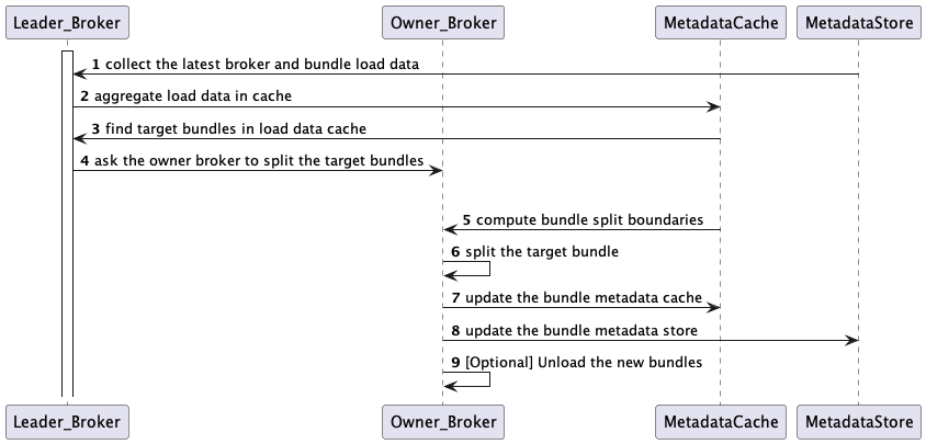
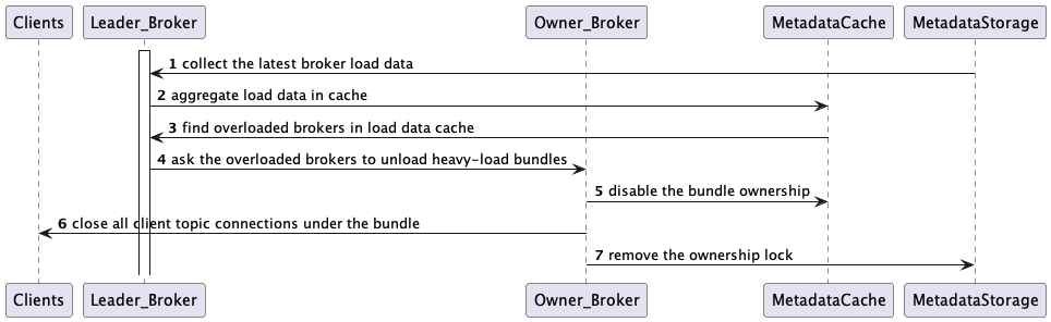 With the broker load information collected from all brokers, the leader broker identifies which brokers are overloaded and triggers bundle unload operations, with the objective of rebalancing the traffic throughout the cluster.
 Read the articles below to learn more:
 Demo Edge Hardware Specifications - 演示使用的边缘端硬件规格
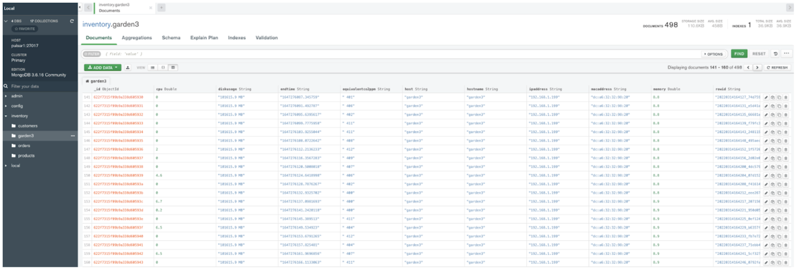
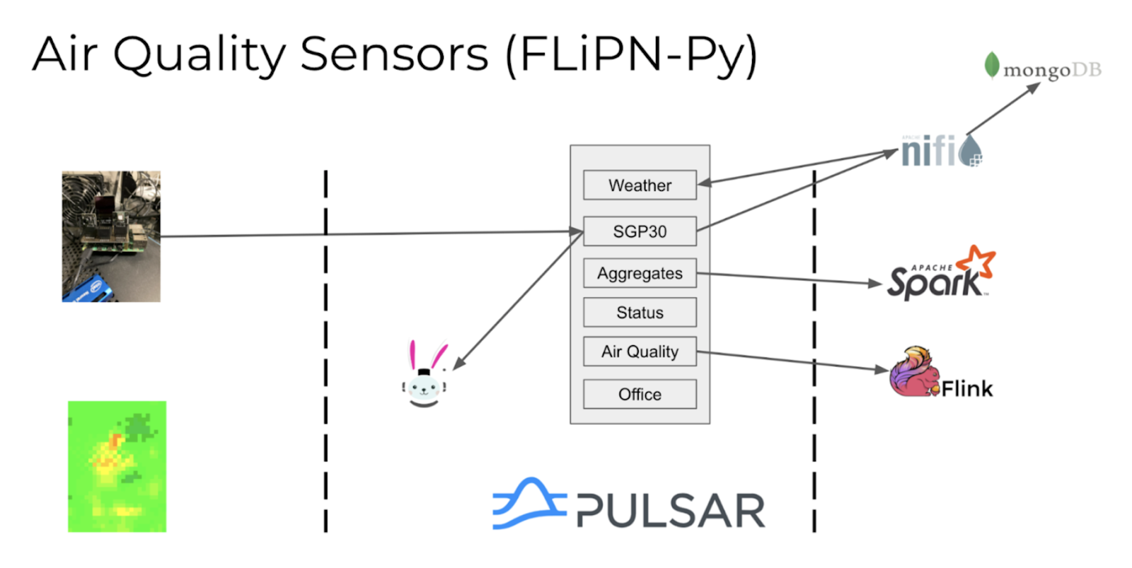 In this application, we want to monitor the air quality in an office continuously and then hand off a large amount of data to a data scientist to make predictions. Once that model is done, we will add that model to a Pulsar function for live anomaly detection to alert office occupants of the situation. We will also want dashboards to monitor trends, aggregates and advanced analytics.


 We can see the broker entry metadata is stored in bookies, but is not visible to a Pulsar consumer.
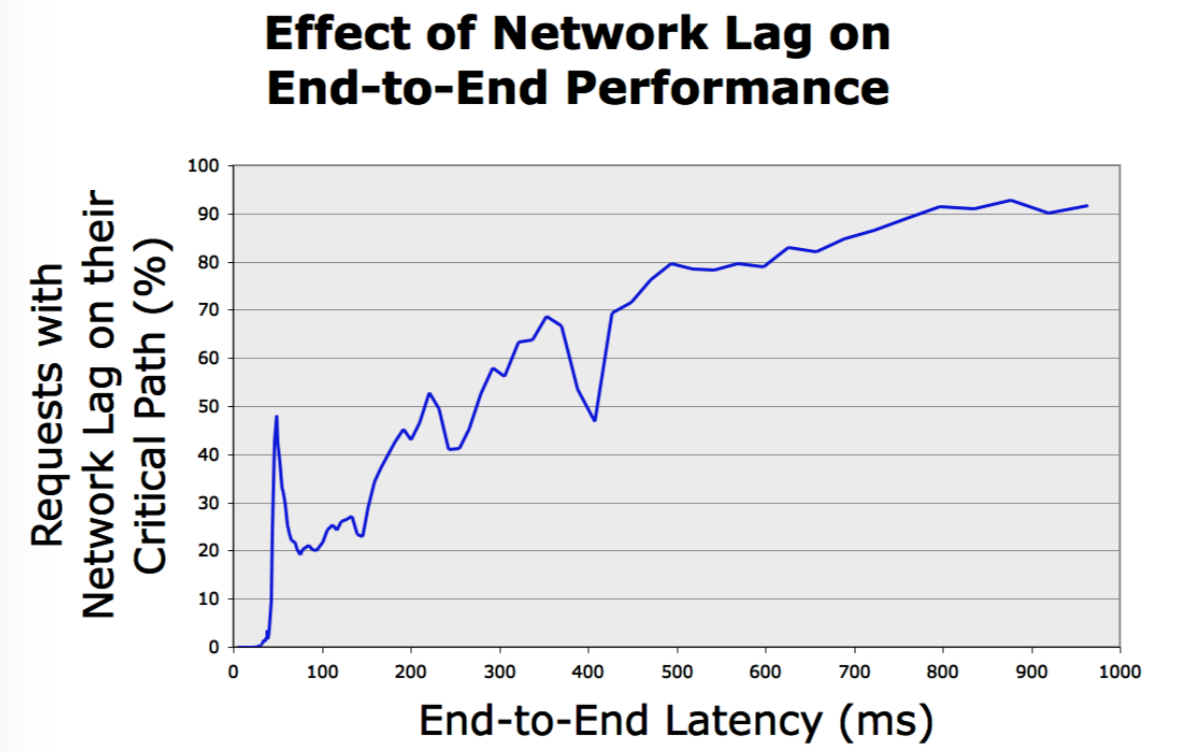 (图-7. 关键路径上遇到非正常网络延迟的全文搜索跟踪,与端到端请求延迟的关系)
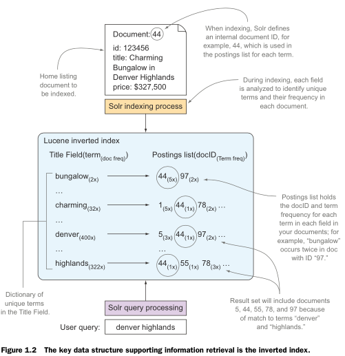
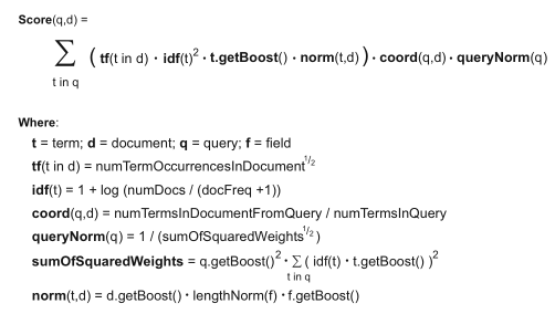
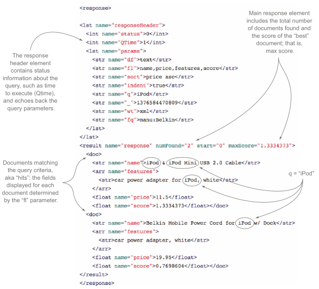 返回结果是按照score排序的:Ranked retrieval。
除非指定了sort参数。
返回结果是按照score排序的:Ranked retrieval。
除非指定了sort参数。